A single DIII-D tokamak shot generates 60+ diagnostic channels at 1 kHz or higher. Before any ML model can train on that data, a physicist has to decide where every plasma event begins and ends — across every channel simultaneously.
How do you label plasma diagnostic data for machine learning? You preprocess all diagnostic channels onto a common time grid, manually label ELM events and plasma regime transitions on a representative set of shots, train an ONNX classifier on those seed labels, then bulk-autolabel hundreds of remaining shots with human review on low-confidence predictions. Full provenance tracking at every step ensures reproducibility.
What Makes Plasma Diagnostic Data Different from Standard Sensor Data
Plasma diagnostic systems do not produce a single CSV you can load into pandas. A tokamak shot produces data from fundamentally different measurement systems: MHD probes capturing magnetic field fluctuations, filterscope arrays measuring line emission intensities, Thomson scattering diagnostics tracking electron temperature and density, and machine control parameters logging coil currents, gas puff timing, and heating power. Each system samples at different rates, starts at different times relative to the discharge, and outputs data in different formats.
The DIII-D tokamak at General Atomics generates 60+ diagnostic channels per shot. MHD probes may sample at 1 MHz during fast instabilities. Filterscope diagnostics may run at 10 kHz. Machine control parameters log at 1 kHz. Thomson scattering fires at discrete time points. Standard time-series tools — built for IoT sensors logging temperature every minute — fail here because they assume homogeneous data: a single sampling rate, a single time base, a single file format. Multimodal plasma diagnostics preprocessing breaks all three assumptions simultaneously.
The shot-based structure compounds the challenge. Every tokamak shot is an independent experiment lasting 2-6 seconds of plasma discharge. A single campaign might produce hundreds of shots over several weeks. Labeling must scale across all of them while remaining consistent enough for a classifier to learn from.
The Preprocessing Foundation: Getting Signals Onto a Common Grid
Before anyone can label anything, every diagnostic channel must exist on the same time axis. This is not optional — it is the foundation without which labeling produces meaningless results.
Step 1: Trim to the plasma window. Raw diagnostic files include pre-shot calibration and post-shot decay. Trim every channel to the same plasma window — typically defined by plasma current exceeding a threshold.
Step 2: Fill probe gaps. MHD probes occasionally drop samples during fast transients. Fill strategies matter: forward-fill preserves causality; linear interpolation works for slow-varying quantities. Never interpolate across event boundaries — if an ELM happened during the gap, filling with averaged values destroys the signal you are trying to label.
Step 3: Resample to a common grid. The DIII-D workflow resamples all diagnostics to the machine control rate (typically 1 kHz). Downsampling high-rate probes requires anti-aliasing filters to avoid introducing spurious frequency content. The choice of target rate determines what phenomena you can resolve: 1 kHz captures most confinement-relevant dynamics; 100 kHz may be required for fast instability analysis.
Step 4: Smooth where appropriate. Savitzky-Golay filtering on noisy magnetic probe signals reduces high-frequency noise while preserving edge structure. Smoothing must happen after resampling — otherwise you are smoothing at the wrong effective frequency.
Step 5: Normalize across diagnostics. MHD probe signals and filterscope intensities live on completely different scales. Z-score or min-max normalization per channel ensures that downstream classifiers weight diagnostics by information content, not by arbitrary signal amplitude. Normalization should be the final preprocessing step — applied after the physics-preserving operations (trim, fill, resample, smooth) are locked in.
The order of these operations is not arbitrary. Resampling before trimming wastes compute. Smoothing before resampling smears information at the wrong scale. Normalizing before smoothing distorts the filter response. A visual DAG makes this ordering explicit and replayable — dFL stores the full operation sequence as an auditable provenance graph. For more on why preprocessing order matters for ML pipelines, see the guide on preprocessing order in time-series ML pipelines.
Manual Labeling of ELMs and Plasma Regime Transitions
ELMs (Edge Localized Modes) are quasi-periodic plasma instabilities — sharp bursts in edge diagnostics: sudden spikes in D-alpha emission, drops in edge electron temperature, and magnetic field perturbations. Labeling them means marking the onset and termination of each event across the relevant channels.
The difficulty is not finding the biggest ELMs. The difficulty is consistent boundary definition across thousands of events. Does the label include the precursor oscillation, or only the crash? Does the recovery period count? A classifier trained on inconsistent boundaries produces inconsistent predictions.
The solution is a reusable label template. Define the ELM class once — onset criterion, termination criterion, which channels to span — and apply that template consistently across shots. In dFL, label templates save this logic so the boundary definition stays fixed from the first shot to the last.
Plasma regime transitions — L-mode to H-mode, or H-mode back to L-mode — require a different approach. These are longer-duration events defined by changes in confinement quality. Mark them as span labels covering the transition period, not point labels on a single moment.
Practical workflow: manually label 10-15 shots covering the operating space you care about. Include clean H-modes, ELM-free periods, frequent ELMs, and confinement degradation. These become the seed labels for autolabeling. For more on the manual-to-automated transition, see the guide on labeling time-series data at scale.
Autolabeling at Scale: From 10 Shots to Hundreds
Manual labeling 200 tokamak shots is not realistic for a research team with deadlines. The autolabel loop:
Seed labels. Manually label ELMs and plasma transitions on 10-15 representative shots. Cover edge cases — not just textbook ELMs, but ELM-like artifacts that should not be labeled.
Train the classifier. Export labeled time windows. Train a simple classifier — even a decision tree or small convolutional network works for ELM detection. Export to ONNX format for deployment into your labeling environment.
Bulk autolabel. Run the ONNX model across all remaining shots. High-confidence predictions (>0.95) are auto-accepted. Low-confidence predictions (<0.70) go to a human review queue. The middle band (0.70-0.95) can be reviewed selectively based on available time — prioritize shots with unusual plasma conditions.
Active learning. Review and correct low-confidence predictions. These corrections become new training data. Retrain. Repeat until the model handles genuinely ambiguous cases reliably. Each iteration tightens the boundary between “clear ELM” and “not an ELM” — the cases that matter most for classifier performance.
dFL’s Autolabel SDK supports this workflow natively: drop in an ONNX model, set confidence thresholds, and the system handles batching, progress tracking, and provenance logging. Every autolabeled event carries metadata — model version, confidence score, parameters. The full technical workflow for building this pipeline is detailed in the autolabeling pipeline guide [internal link -> /sensor-data-autolabeling-pipeline-onnx-python/].
The productivity gain is measurable. A physicist who might spend days manually labeling ELMs across a shot campaign can complete the same work in hours — with better consistency, because the classifier applies the same boundary logic to every event.
Provenance for Plasma Diagnostics: Why Reproducibility Is Non-Negotiable
“Before dFL, we were spending 2-3 weeks per shot campaign just figuring out what preprocessing we’d done six months ago. Now that’s a five-minute DAG review.”
Fusion research teams increasingly operate under FAIR data requirements from DOE Fusion Energy Sciences and other funding agencies. A Jupyter notebook with ad-hoc preprocessing cells does not meet FAIR’s reproducibility standard. A structured provenance DAG does.
The provenance DAG records: raw data sources and ingestion parameters, each preprocessing operation with exact parameters and execution order, which autolabeler version was applied with what confidence threshold, every human label (author, timestamp, class, span boundaries), and every human correction to autolabeled events.
In dFL, this record exports as JSON. Send it to a collaborator at PPPL or LANL. They load the same raw files, apply the same DAG, and get the identical labeled dataset. No guesswork. No data archaeology. When multiple researchers label concurrently — common in multi-institution collaborations — each edit carries author attribution, so disagreements surface as visible diffs rather than silent overwrites.
The full provenance framework, including FAIR compliance mapping and ISO 8000 traceability requirements, is covered in the sensor data provenance guide [internal link -> /sensor-data-provenance-ml-pipelines/].
Tooling That Handles Fusion Data: What to Look For
Most time-series tools were not built for plasma diagnostic complexity. Industrial analytics platforms like Seeq and TrendMiner assume historian-rate data (seconds between samples) and do not offer DSP preprocessing depth. General-purpose labeling platforms like Scale AI and Labelbox focus on images, text, and video — not multimodal sensor streams at kHz rates. MATLAB Signal Labeler offers DSP depth but is single-user, license-bound, and MATLAB-only.
Before evaluating labeling platforms for plasma diagnostic data, confirm five requirements:
- High-rate capability (kHz+). Interactive pan/zoom at 1 kHz with 60+ channels is the minimum bar.
- Multi-channel concurrent visualization. See MHD probes, filterscope, and machine control parameters simultaneously on the same time axis.
- DSP preprocessing built in. Trim, fill, resample, smooth, normalize — in a visual interface, not separate scripts.
- Autolabel SDK with ONNX support. Plug in custom classifiers trained in PyTorch, TensorFlow, or scikit-learn via ONNX.
- Full provenance DAG with on-prem deployment. Research institutions often require on-prem data handling. The provenance system must export to open formats (JSON), not proprietary databases.
dFL meets all five. The DIII-D tokamak workflow was one of the earliest use cases, and the architecture reflects that origin. 60+ channels at 1 kHz+ is the design target, not a stress test. For a full comparison across these dimensions, see the 2026 time-series labeling tools buyer’s guide.
FAQ
What sampling rate do tokamak diagnostic systems use?
It varies by diagnostic. Machine control parameters typically log at 1 kHz. Filterscope and bolometry may run at 10-100 kHz. Fast magnetic probes for MHD analysis can exceed 1 MHz. A practical workflow resamples everything to a common rate — often the machine control rate — for cross-diagnostic analysis, while preserving access to high-rate raw data for fast-transient studies.
Can you autolabel ELMs without manual examples?
No. The classifier needs to learn what an ELM looks like in your specific diagnostic configuration. ELMs in a high-field compact tokamak look different from ELMs in a large conventional tokamak. Manual seed labels — even 50-100 examples — are required to train a useful classifier. The seed set should include clear ELMs, ambiguous events, and non-ELM artifacts so the model learns all three categories.
What file formats do plasma diagnostic systems export?
MDSplus is the de facto standard for US fusion experiments. HDF5 is common for international machines. Some smaller experiments use CSV or custom binary formats. dFL’s Data Provider architecture supports custom Python ingestion scripts — write a script that reads your format, and the platform handles everything downstream.
How does dFL handle 60+ channel fusion data?
Multiple graphs per tab, multiple tabs per project, concurrent visualization of as many signals as your screen can display. The visual DAG applies the same preprocessing sequence to all loaded records. Bulk export produces harmonized datasets with consistent preprocessing across all channels.
How do fusion research teams handle preprocessing reproducibility?
Most teams rely on Jupyter notebooks or custom scripts, which break when data formats change or team members leave. A provenance DAG solves this by recording every preprocessing decision — parameters, order of operations, author — as a replayable graph. In dFL, the entire DAG exports as JSON and can be reapplied to new raw data by any team member, at any institution, months or years later.
- The DIII-D plasma team processes 60+ channels at 1 kHz+ in dFL. Try it free with your own shot data.
- For the full methodology paper on dFL’s architecture and provenance system, read our paper